Exploring the Jaynes-Cummings Model
The Jaynes-Cummings model is a compact example of a system containing both a
two-level degree of freedom and a harmonic oscillator. It is therefore a useful
test case for the two directions supported by second_quantization:
- Construct a symbolic Hamiltonian and convert it to a numerical matrix.
- Recover a normal-ordered symbolic expression from that matrix.
In this tutorial, we build the Jaynes-Cummings Hamiltonian, validate the bosonic and mixed fermion-boson conversions, compare its spectrum with the analytic result, and use a parameter sweep to explore the hybridized spectrum.
# Symbolic tools
import sympy
from sympy.physics.quantum import Dagger
from sympy.physics.quantum.boson import BosonOp
from sympy.physics.quantum.fermion import FermionOp

# Numerical tools
import numpy as np
import matplotlib.pyplot as plt

# Second-quantization package
from second_quantization import hilbert_space
Defining the Jaynes-Cummings Hamiltonian
We represent the qubit with one fermionic mode c and the resonator with one
bosonic mode a. The fermionic vacuum is the qubit ground state, so
sigma_z = 2 c^dagger c - 1.
With this convention, the Jaynes-Cummings Hamiltonian is
$$ H_{\mathrm{JC}} = \frac{\omega_q}{2}\sigma_z + \omega_r a^\dagger a + g\left(c^\dagger a + c a^\dagger\right), $$
where omega_q and omega_r are the qubit and resonator frequencies and g
is their coupling.
# Symbolic operators
c = FermionOp("c")
a = BosonOp("a")
operators = [c, a]

# Symbolic parameters
omega_q, omega_r, g = sympy.symbols("omega_q omega_r g", real=True)

# Qubit Pauli operator in fermionic language
sigma_z = 2 * Dagger(c) * c - 1

# Jaynes-Cummings Hamiltonian
hamiltonian = (
    omega_q / 2 * sigma_z
    + omega_r * Dagger(a) * a
    + g * (Dagger(c) * a + c * Dagger(a))
)

sympy.Eq(sympy.Symbol(r"H_{\mathrm{JC}}"), hamiltonian.expand())
$\displaystyle H_{\mathrm{JC}} = g {{c}^\dagger} {a} + g {c} {{a}^\dagger} - \frac{\omega_{q}}{2} + \omega_{q} {{c}^\dagger} {c} + \omega_{r} {{a}^\dagger} {a}$
From a symbolic expression to a numerical matrix
Bosons have infinitely many occupation states, so every numerical calculation
must specify a truncation. Here truncation = 10 retains the states
|0> through |10> for the resonator. With one fermion and one boson, the
matrix dimension is 2 * (truncation + 1).
to_matrix returns a dictionary rather than immediately substituting symbolic
parameters. Its keys are the symbolic prefactors and its values are the
corresponding matrices. make_dict_callable turns that dictionary into a
fast function for evaluating many parameter sets.
truncation = 10

matrix_terms = hilbert_space.to_matrix(
    hamiltonian,
    operators=operators,
    sparse=False,
    truncation=truncation,
)
hamiltonian_func = hilbert_space.make_dict_callable(matrix_terms)

parameters = dict(omega_q=1.0, omega_r=1.0, g=0.2)
matrix = hamiltonian_func(**parameters)

print("Symbolic prefactors:", list(matrix_terms))
print("Hilbert-space dimension:", matrix.shape[0])
Symbolic prefactors: [omega_q, g, omega_r]
Hilbert-space dimension: 22
The returned matrix uses the tensor-product ordering set by operators:
fermions first, then bosons. Keeping the same ordered list is essential when
converting a matrix back into operators.
Validating the bosonic inverse
Before using a mixed system, we can test the bosonic inversion on expressions whose matrix representation we construct ourselves. A round trip should reproduce the original matrix. Comparing matrices is the appropriate check: algebraically equivalent symbolic expressions need not have identical printed forms.
def round_trip(expression, operator_list, truncation):
    """Convert a numeric expression to a matrix and back again."""
    original_terms = hilbert_space.to_matrix(
        expression,
        operators=operator_list,
        sparse=False,
        truncation=truncation,
    )
    original_matrix = sum(original_terms.values())

    recovered_expression = hilbert_space.to_operators(
        original_matrix,
        basis=operator_list,
        truncation=truncation,
    )
    recovered_terms = hilbert_space.to_matrix(
        recovered_expression,
        operators=operator_list,
        sparse=False,
        truncation=truncation,
    )
    recovered_matrix = sum(recovered_terms.values())

    error = np.max(np.abs(original_matrix - recovered_matrix))
    return recovered_expression, error


boson_expressions = [
    a,
    Dagger(a),
    Dagger(a) * a,
    Dagger(a) ** 2 * a**2 + Dagger(a) * a + sympy.Rational(1, 3),
    Dagger(a) + a,
]

for expression in boson_expressions:
    recovered, error = round_trip(expression, [a], truncation=6)
    print(f"{expression!s:45} error = {error:.2e}")
a                                             error = 0.00e+00
Dagger(a)                                     error = 0.00e+00
Dagger(a)*a                                   error = 0.00e+00
1/3 + Dagger(a)*a + Dagger(a)**2*a**2         error = 0.00e+00
Dagger(a) + a                                 error = 0.00e+00
The same routine applies to multiple bosonic modes. In this example, a and
b are different resonator modes and have independent cutoffs.
b = BosonOp("b")

two_mode_expression = (
    Dagger(a) * b
    + Dagger(b) * a
    + sympy.Rational(1, 4) * Dagger(a) * a * Dagger(b) * b
)
recovered, error = round_trip(two_mode_expression, [a, b], truncation=[4, 4])

print("Recovered expression:")
sympy.pprint(recovered)
print(f"Maximum matrix error: {error:.2e}")
Recovered expression:
 †    †
a ⋅a⋅b ⋅b    †        †
───────── + a ⋅b + a⋅b
    4
Maximum matrix error: 0.00e+00
Recovering the mixed Hamiltonian
We can now invert the numerical Jaynes-Cummings matrix. The basis argument
must match the operator list used by to_matrix, and the bosonic truncation
must be supplied again. to_operators returns a normal-ordered SymPy
expression with numerical coefficients.
recovered_hamiltonian = hilbert_space.to_operators(
    matrix,
    basis=operators,
    truncation=truncation,
)
recovered_terms = hilbert_space.to_matrix(
    recovered_hamiltonian,
    operators=operators,
    sparse=False,
    truncation=truncation,
)
recovered_matrix = sum(recovered_terms.values())

round_trip_error = np.max(np.abs(matrix - recovered_matrix))

print("Recovered Hamiltonian:")
sympy.pprint(recovered_hamiltonian)
print(f"Maximum matrix error: {round_trip_error:.2e}")
assert round_trip_error < 1e-10
Recovered Hamiltonian:
  1    †          †      †            †
- ─ + a ⋅a + 0.2⋅c ⋅a + c ⋅c + 0.2⋅c⋅a
  2
Maximum matrix error: 0.00e+00
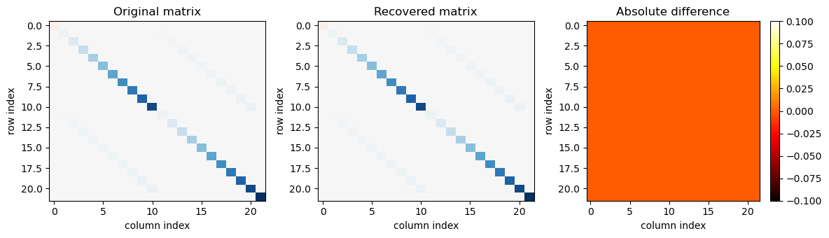
The following plot makes the same check visually. The final panel should be zero up to numerical roundoff.
fig, axes = plt.subplots(1, 3, figsize=(12, 3.5))

color_limits = dict(
    cmap="RdBu",
    aspect="auto",
    vmin=-np.max(np.abs(matrix)),
    vmax=np.max(np.abs(matrix)),
)

axes[0].imshow(matrix.real, **color_limits)
axes[0].set_title("Original matrix")

axes[1].imshow(recovered_matrix.real, **color_limits)
axes[1].set_title("Recovered matrix")

difference = axes[2].imshow(
    np.abs(matrix - recovered_matrix),
    cmap="hot",
    aspect="auto",
)
axes[2].set_title("Absolute difference")
fig.colorbar(difference, ax=axes[2])

for axis in axes:
    axis.set_xlabel("column index")
    axis.set_ylabel("row index")

plt.tight_layout()
plt.show()
Checking the analytic spectrum
The fermionic encoding also gives a useful physics check. Let
delta = omega_q - omega_r. The vacuum |g, 0> has energy
$$ E_0 = -\frac{\omega_q}{2}. $$
For each excitation number $n \geq 1$, the coupled states
|g, n> and |e, n - 1> have energies
$$ E_{n,\pm} = \left(n - \frac{1}{2}\right)\omega_r \pm \sqrt{\left(\frac{\delta}{2}\right)^2 + g^2 n}. $$
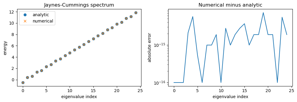
At a finite bosonic cutoff, the highest state has no partner above the cutoff. We therefore compare the vacuum and the complete coupled doublets up to the cutoff.
def analytic_energies(omega_q, omega_r, coupling, truncation):
    """Return the vacuum and Jaynes-Cummings doublets below the cutoff."""
    delta = omega_q - omega_r
    energies = [-omega_q / 2]

    for n in range(1, truncation + 1):
        average = (n - 0.5) * omega_r
        splitting = np.sqrt((delta / 2) ** 2 + coupling**2 * n)
        energies.extend([average - splitting, average + splitting])

    return np.sort(energies)


spectrum_truncation = 12
spectrum_parameters = dict(omega_q=1.0, omega_r=1.0, g=0.1)

spectrum_terms = hilbert_space.to_matrix(
    hamiltonian,
    operators=operators,
    sparse=False,
    truncation=spectrum_truncation,
)
spectrum_func = hilbert_space.make_dict_callable(spectrum_terms)
numeric_energies = np.sort(np.linalg.eigvalsh(spectrum_func(**spectrum_parameters)))
expected_energies = analytic_energies(
    spectrum_parameters["omega_q"],
    spectrum_parameters["omega_r"],
    spectrum_parameters["g"],
    spectrum_truncation,
)

spectral_error = np.max(
    np.abs(numeric_energies[: len(expected_energies)] - expected_energies)
)
print(f"Maximum eigenvalue error: {spectral_error:.2e}")
assert spectral_error < 1e-10
Maximum eigenvalue error: 7.11e-15
fig, axes = plt.subplots(1, 2, figsize=(10, 3.5))

axes[0].plot(expected_energies, "o", label="analytic")
axes[0].plot(numeric_energies[: len(expected_energies)], "x", label="numerical")
axes[0].set_xlabel("eigenvalue index")
axes[0].set_ylabel("energy")
axes[0].set_title("Jaynes-Cummings spectrum")
axes[0].legend()

axes[1].semilogy(
    np.abs(numeric_energies[: len(expected_energies)] - expected_energies) + 1e-16
)
axes[1].set_xlabel("eigenvalue index")
axes[1].set_ylabel("absolute error")
axes[1].set_title("Numerical minus analytic")

plt.tight_layout()
plt.show()
Exploring the detuning
The symbolic conversion above happens only once. The callable
hamiltonian_func then evaluates the same operator structure at each parameter
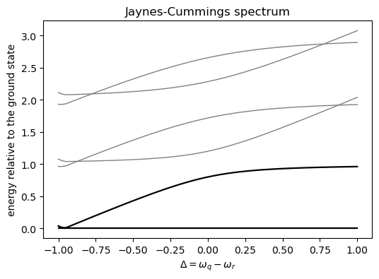
set, which makes it natural to explore how the spectrum changes with detuning
Delta = omega_q - omega_r.
The first excited doublet exhibits an avoided crossing near Delta = 0. At
resonance, its splitting is approximately 2 g, the vacuum Rabi splitting.
omega_r_value = 1.0
coupling_value = 0.2
detunings = np.linspace(-1.0, 1.0, 81)
levels = []

for detuning in detunings:
    spectrum_matrix = hamiltonian_func(
        omega_q=omega_r_value + detuning,
        omega_r=omega_r_value,
        g=coupling_value,
    )
    eigenvalues = np.linalg.eigvalsh(spectrum_matrix)
    levels.append(eigenvalues[:6] - eigenvalues[0])

levels = np.array(levels)

fig, ax = plt.subplots(figsize=(6, 4))
for level in range(levels.shape[1]):
    color = "black" if level < 2 else "gray"
    linewidth = 1.6 if level < 2 else 1.0
    ax.plot(detunings, levels[:, level], color=color, linewidth=linewidth)

ax.set_xlabel(r"$\Delta = \omega_q - \omega_r$")
ax.set_ylabel("energy relative to the ground state")
ax.set_title("Jaynes-Cummings spectrum")
plt.show()
Summary
This tutorial used the Jaynes-Cummings model to show that
second_quantization can:
- represent fermions and bosons in one ordered Hilbert space;
- convert a parameterized symbolic Hamiltonian into dense or sparse matrices;
- reconstruct normal-ordered bosonic and mixed operator expressions; and
- validate the result against both the original matrix and an analytic spectrum;
- reuse the symbolic Hamiltonian to explore spectra across a parameter sweep.